Demystify Machine Learning - Random Forest

This could be the age of LLM’s but understanding classical ML and under-the-hood workings never gets old and goes a long way in implementing real-world projects, especially for tabular data.

One vital class of Machine Learning is Supervised learning which aims at learning a function that maps an input to an output based on example input-output pairs. One such popular algorithm under the Supervised branch is Random Forest.

Random forests are an ensemble learning method for classification, regression and other tasks that operates by constructing a multitude of decision trees at training time and outputting the class that is the mode of the classes (classification) or mean prediction (regression) of the individual trees.

But how do these work under the hood? Understanding underlying workings is important for a Data Scientist/ML Engineer as even a basic algorithm can solve a customer’s problem and after a point, it is the understanding of the algorithm that will improve the solution to the customer’s problem.

Let’s look at one of the ways to understand Decision Trees and Random Forest predictions and see how the prediction is arrived at for each observation.

NOTE:

1) This Package works only with scikit-learn modules.

2) To install tree interpreter run, “pip install treeinterpreter“. Refer https://github.com/andosa/treeinterpreter

So, where do we start?

We start by looking at decision trees which are the building blocks of random forest.

How do decision trees work?

A Decision Tree is a tree (and a type of directed, acyclic graph) in which the nodes represent decisions (a square box), random transitions (a circular box) or terminal nodes, and the edges or branches are binary (yes/no, true/false) representing possible paths from one node to another. The specific type of decision tree used for machine learning contains no random transitions. To use a decision tree for classification or regression, one grabs a row of data or a set of features and starts at the root, and then through each subsequent decision node to the terminal node. The process is very intuitive and easy to interpret, which allows trained decision trees to be used for variable selection or more generally, feature engineering.

Terminologies in Decision Trees

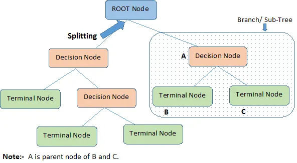
-> Root Node: It represents the entire population or sample and this further gets divided into two or more homogeneous sets.

-> Splitting: It is a process of dividing a node into two or more sub-nodes.

-> Decision Node: When a sub-node splits into further sub-nodes, then it is called a decision node.

-> Leaf/ Terminal Node: Nodes with no children (ie.. no further split) are called a Leaf or a Terminal node.

-> Pruning: When we reduce the size of decision trees by removing nodes (opposite of Splitting), the process is called pruning.

-> Branch / Sub-Tree: A subsection of the decision tree is called a branch or sub-tree.

-> Parent and Child Node: A node, which is divided into sub-nodes is called a parent node of sub-nodes whereas sub-nodes are the child of the parent node

For Classification trees, the splits are chosen so as to;

1) Minimize Entropy or 2) Minimize Gini impurity in the Resulting Subsets.

An example of a learned decision tree for classification to help you make your decision is below;

The Core Algorithm of a Decision Tree is ID3 and it uses Entropy and Information Gain to construct a decision tree. ID3 algorithm uses entropy to calculate the homogeneity of a sample. Information theory/Gain is a measure to define the degree of disorganization in a system known as Entropy.

If the sample is completely homogeneous, then the entropy is zero and if the sample is equally divided (50% — 50%), it has an entropy of one.

\[Entropy = -p \log_2 p - q \log_2 q\]

Here p and q are the probability of success and failure respectively in that node. Entropy is also used with the categorical target variable. It chooses the split which has the lowest entropy compared to the parent node and other splits. The lesser the entropy, the better it is.

Steps to Calculate Entropy:

1) Calculate the entropy of the parent node.

2) Calculate the entropy of each individual node of split and calculate the weighted average of all sub-nodes available in the split.

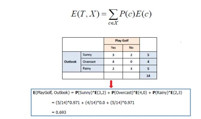
Information Gain

Information Gain, on the other hand, is all about finding an attribute that returns the highest value( homogeneous branches)

Step 1: Calculate the entropy of the target.

Step 2: The dataset is then split into the different attributes. The entropy for each branch is calculated. Then it is added proportionally, to get the total entropy for the split. The resulting entropy is subtracted from the entropy before the split. The result is the Information Gain or decrease in entropy.

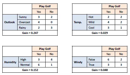
Step 3: Choose the attribute with the largest information gain as the decision node, divide the dataset by its branches and repeat the same process on every branch.

So, in the above situation, we choose the Outlook attribute as that has the highest gain value.

Gini Index

The Gini index which is different than the Gini Impurity says, that if we select two items from a population at random then they must be of the same class and the probability for this is 1 if the population is pure.

Steps to calculate Gini for a split:

1) Calculate Gini for sub-nodes, using the formula - the sum of the square of probability for success and failure (p^2+q^2).

2) Calculate the Gini for the split using the weighted Gini score of each node of that split.

\[Gini = 1 - \sum_{i=1}^{n} p_i^2\]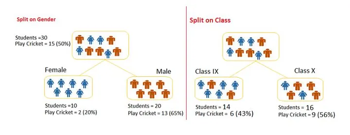

Split on Gender:

1. Gini for sub-node Female = (0.2)(0.2)+(0.8)(0.8)=0.68
2. Gini for sub-node Male = (0.65)(0.65)+(0.35)(0.35)=0.55
3. Weighted Gini for Split Gender = (10/30)0.68+(20/30)0.55 = 0.59

Split on Class:

1. Gini for sub-node Class IX = (0.43)(0.43)+(0.57)(0.57)=0.51
2. Gini for sub-node Class X = (0.56)(0.56)+(0.44)(0.44)=0.51
3. Weighted Gini for Split Class = (14/30)0.51+(16/30)0.51 = 0.51

As you can see above, the value is higher for Gender and therefore the split will occur on the Gender attribute.

Chi-Square

Another method to find the best split for classification problems is chi-square. Let’s take a brief look at that.

It is an algorithm to find out the statistical significance of the differences between sub-nodes and parent nodes. We measure it by the sum of squares of standardised differences between observed and expected frequencies of the target variable.

The higher the value of Chi-Square, the higher the statistical significance of differences between sub-node and Parent node.

Chi-square = ((Actual — Expected)² / Expected)¹/2

Steps to Calculate Chi-square for a split

1. Calculate the Chi-square for an individual node by calculating the deviation for the Success and Failure of both.
2. Calculated Chi-square of the Split using the Sum of all Chi-square of success and Failure of each node of the split

Using the same dataset, splitting on Gender:

1. First, we are populating for node Female, Populate the actual value for “Play Cricket” and “Not Play Cricket”, here these are 2 and 8 respectively.
2. Calculate the expected value for “Play Cricket” and “Not Play Cricket”, here it would be 5 for both because the parent node has a probability of 50% and we have applied the same probability on the Female count(10).
3. Calculate deviations by using the formula, Actual — Expected. It is for “Play Cricket” (2–5 = -3) and for “Not play cricket” ( 8–5 = 3).
4. Calculate the Chi-square of a node for “Play Cricket” and “Not Play Cricket” using the formula with formula, = ((Actual — Expected)² / Expected)¹/2. You can refer to the below table for the calculation.
5. Follow similar steps for calculating the Chi-square value for the Male node.
6. Now add all Chi-square values to calculate the Chi-square for split Gender.

Splitting on class gives you the below table

Which tree algorithm does scikit-learn use? CART it is, more on that on the scikit learn page.

So far what we saw, applies to classification problems. Most ML frameworks(like scikit-learn) by default uses the variance approach as the splitting criteria for regression problems. There are 2 approaches to choose from for regression problems.

For regression trees, they are either chosen to minimize Variance (Reduction in Variance approach) OR MAE (Mean Absolute Error) within all of the subsets.

Variance (Reduction in Variance approach)

This algorithm uses the standard formula of variance to choose the best split. The split with lower variance is selected as the criteria to split the population.

\[Variance = \frac{\sum_ (x - \bar{x})^2} {n}\]

Steps to calculate Variance:

1. Calculate the variance for each node.
2. Calculate variance for each split as the weighted average of each node variance.

Example:- Let us assign numerical value 1 for playing cricket and 0 for not playing cricket. Now follow the steps to identify the right split:

1. Variance for the Root node, the mean value is (151 + 150)/30 = 0.5 and we have 15 one and 15 zero. Now variance would be ((1–0.5)²+(1–0.5)²+….15 times+(0–0.5)²+(0–0.5)²+…15 times) / 30, this can be written as (15(1–0.5)²+15(0–0.5)²) / 30 = 0.25

2. Mean of Female node = (21+80)/10=0.2 and Variance = (2(1–0.2)²+8(0–0.2)²) / 10 = 0.16

3. Mean of Male Node = (131+70)/20=0.65 and Variance = (13(1–0.65)²+7(0–0.65)²) / 20 = 0.23

4. Variance for Split Gender = Weighted Variance of Sub-nodes = (10/30)*0.16 + (20/30) *0.23 = 0.21

5. Mean of Class IX node = (61+80)/14=0.43 and Variance = (6(1–0.43)²+8(0–0.43)²) / 14= 0.24

6. Mean of Class X node = (91+70)/16=0.56 and Variance = (9(1–0.56)²+7(0–0.56)²) / 16 = 0.25

7. Variance for Split Gender = (14/30)*0.24 + (16/30) *0.25 = 0.25

Above, you can see that the Gender split has a lower variance compared to the parent node, so the split would take place on the Gender variable.

So far we have seen some theories behind decision trees and how they work. Let us look at some code examples to see how a prediction/decision is arrived at.

Implementing Decision Tree

NOTE: Codes seen here were executed on Kaggle. It is posted here only for the purpose of understanding the concepts talked about in this post.

Let us look at a housing dataset where the target variable is Price. We need to predict the price of the house given other variables like square feet, latitude/longitude of the house, no. of bedrooms etc. You can access the dataset here.

import pandas as pd
import numpy as np
from treeinterpreter import treeinterpreter as ti
from sklearn.tree import DecisionTreeRegressor
from sklearn.ensemble import RandomForestRegressor
rf = RandomForestRegressor()
dt = DecisionTreeRegressor()
y = data.iloc[:,2]
x = data.loc[:, data.columns != 'price']
x = x.drop('date',1)
x = x.drop('id', 1)
from sklearn.model_selection import train_test_split
X_train, X_test, y_train, y_test = train_test_split(x, y, test_size=0.33, random_state=42)

dt.fit(X_train, y_train)
## Looking at a single instance
instances = X_test.loc[[735]]
instances

Turning a Black-box into an interpretable model using Treeinterpreter.

prediction, bias, contributions = ti.predict(dt, instances)
## Feature Contributions
ft_list = []
for i in range(len(instances)):
    #print("Instance", i)
    print("Bias (trainset mean)", bias[i])
    #print("Feature contributions:")
    for c, feature in sorted(zip(contributions[i], 
                                 x.columns), 
                             key=lambda x: -abs(x[0])):
       ft_list.append((feature, round(c, 2)))
    print("-"*50)

## OUTPUT:
## Bias (trainset mean) 537789.045718232
labels, values = zip(*ft_list)
## Let us look at feature coefficients
ft_list
[('lat', -98263.16),
 ('sqft_living', 97872.84),
 ('grade', -53306.67),
 ('long', -45117.71),
 ('view', -15900.9),
 ('sqft_living15', -12963.56),
 ('yr_built', 5982.33),
 ('sqft_above', -5913.17),
 ('sqft_basement', -4933.08),
 ('sqft_lot', -3708.75),
 ('sqft_lot15', -1537.2),
 ('bedrooms', 0.0),
 ('bathrooms', 0.0),
 ('floors', 0.0),
 ('waterfront', 0.0),
 ('condition', 0.0),
 ('yr_renovated', 0.0),
 ('zipcode', 0.0)]

What do these results mean you may ask?

The Treeinterpreter library decomposes the predictions as the sum of contributions from each feature. ie.

Prediction = bias + feature(1) Contribution + …. + feature(n)Contribution

Here are the contributions of all features for instance 735 from the test set.

contributions

## output:
array([[     0.        ,      0.        ,  97872.83764256,
         -3708.75      ,      0.        ,      0.        ,
        -15900.90137409,      0.        , -53306.6745909 ,
         -5913.17280165,  -4933.08088235,   5982.32648995,
             0.        ,      0.        , -98263.16125045,
        -45117.71012643, -12963.55960952,  -1537.19921534]])

Similarly, you can view prediction and bias value made by the decision tree classifier.

prediction
array([400000.])

bias
array([537789.04571823])

Therefore, the prediction must equal,

print(bias + np.sum(contributions, axis=1))
[400000.]

As seen in the coefficients above, only 2 features have a positive impact on driving the prices higher. The feature contributions are sorted by their absolute impact. We can see that in the instance the predicted value is lower than the data set mean and that latitude has a negative impact, the square foot has a high positive impact meaning, the higher the sqft. higher the price, which makes sense.

But this is not where it stops, you might want to know how the Decision tree arrives at its results. For that, we are going to fit a few rows and check the results for it.

top50x = X_train.head(50)
top5x = X_train.head(5)
top50y = y_train.head(50)
top5y = y_train.head(5)
dt1 = DecisionTreeRegressor()
dt1.fit(top5x, top5y)
from sklearn.externals.six import StringIO  
from IPython.display import Image  
from sklearn.tree import export_graphviz
import pydotplus
dot_data = StringIO()
export_graphviz(dt1, out_file=dot_data,  
                filled=True, rounded=True,
                special_characters=True)
graph = pydotplus.graph_from_dot_data(dot_data.getvalue())
  
Image(graph.create_png())

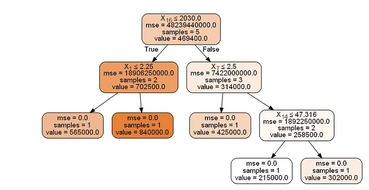
Let us look at the train set and its corresponding target for clarity purpose and also to confirm if the above tree gives us the same results.

top5x

top5y

You can see that the target values are only from among the terminal node values shown in the Decision Tree Split Figure above.

Now that we know how Decision trees work, it is time to move to part 2 — an advanced technique called the Random Forest.