Demystify Machine Learning - Random Forest - Part 2

Dive into Random Forest

In the previous post, we looked at the fundamentals of Trees, how it is split, how they are calculated and how a classifier arrives at a specific prediction using code examples.

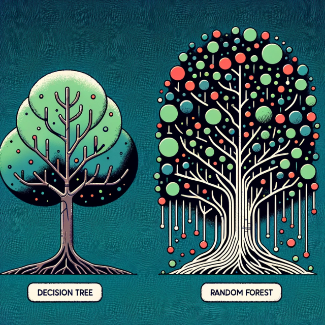
In this post, we go to the next step — An ensemble learning method for classification, regression and other tasks that operates by constructing a multitude of decision trees at training time and outputting the class that is the mode of the classes or mean prediction of the individual trees. Random forest is like a bootstrapping algorithm with a Decision tree (CART) model.

The random forest has been a burgeoning machine learning technique in the last few years. It is a non-linear tree-based model that often provides accurate results. However, being a black box, it is oftentimes hard to interpret and fully understand especially when it comes to explaining the results and rationale behind it to stakeholders in organizations.

From decision trees to forest: We started the previous post with decision trees, so how do we move from a decision tree to a forest?

This is straightforward since the prediction of a forest is the average of the predictions of its trees, the prediction is simply the average of the bias terms plus the average contribution of each feature.

Steps:

1) Assume the number of cases in the training set is N. Then, a sample of these N cases is taken at random but with replacement. This sample will be the training set for growing the tree.

2) If there are M input variables, a number m < M is specified such that at each node, m variables are selected at random out of the M. Among the “m” features, calculate the node “d” using the best split point to split the node. The value of m is held constant while we grow the forest. The nodes are further split into daughter nodes using the best split.

The splitting criteria are similar to that of the decision tree regressor in scikit-learn package.

3) Build a forest by repeating the above steps “n” number of times to create “n” number of trees(n_estimators in sci-kit-learn). Each tree is grown to the largest extent possible and there is no pruning.

4) Predict new data by aggregating the predictions of the ntree( “n” number of trees) trees (i.e., majority votes for classification, the average for regression).

Let us look at implementing those,

rf.fit(X_train, y_train)

Again, turning a black box into a white box for a random forest prediction.

rf_prediction, rf_bias, rf_contributions = ti.predict(rf, instances)
rf_ft_list = []
for i in range(len(instances)):
    print("Bias (trainset mean)", rf_bias[i])
    for c, feature in sorted(zip(rf_contributions[i], 
                                 x.columns), 
                             key=lambda x: -abs(x[0])):
       rf_ft_list.append((feature, round(c, 2)))
    print("-"*50)

rf_labels, rf_values = zip(*rf_ft_list)
rf_ft_list

What does this tell us?

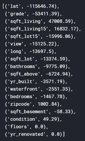
As seen in the results above, 4 features have a positive impact in driving the prices higher, but this time latitude has a very high negative impact, bringing the predictions much less than the bias(trainset mean).

Looking at the contributions, predictions and Bias terms.

rf_contributions

rf_prediction

rf_bias

Again, prediction must equal “ bias + feature(1)contribution + … + feature(n)contribution “.

print(rf_bias + np.sum(rf_contributions, axis=1))

Similar to how we saw in the previous post on how a Decision tree arrived at the results, let us look at a Random Forest arrived at its predictions.

from sklearn.ensemble import RandomForestRegressor
rf_model = RandomForestRegressor(n_estimators=10)
top5xrf = X_train.head(5)
top5yrf = y_train.head(5)
rf_model.fit(top5xrf, top5yrf)

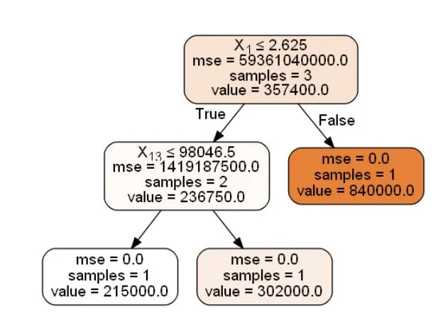
Extracting a single tree to Visualise the results,

estimator = rf_model.estimators_[5]
from sklearn.externals.six import StringIO  
from IPython.display import Image
from sklearn.tree import export_graphviz
import pydotplus
dot_data1 = StringIO()
export_graphviz(estimator, out_file=dot_data1,  
               filled=True, rounded=True,
               special_characters=True)
graph = pydotplus.graph_from_dot_data(dot_data1.getvalue())  
Image(graph.create_png())

Although one image is not going to solve the issue, looking at an individual decision tree shows us that a random forest is not an unexplainable method, but a sequence of logical questions and answers and every prediction can be trivially presented as a sum of features contributions, showing how the features lead to a particular prediction.

This opens up a lot of opportunities in practical machine learning tasks.

I hope this 2-part series sparked some interest towards understanding the underlying workings of ML Algorithms.

If you like the content, consider supporting me!

You could get me a coffee!